Next Processing Steps

Assigning Species IDs

PAMpal supports a variety of ways to assign species identifications to specific AcousticEvent objects. These IDs can then be used for filtering data or potentially exporting to create a BANTER model. Species assignment is always done using the setSpecies function, and has three possible modes of operation that can be selected using the method argument.

For method='pamguard', species IDs will be assigned according to the labels set in Pamguard for each event. This will only work for AcousticStudy objects created by processPgDetections using mode='db'. For events created using the Click Detector module (these have prefix OE in PAMpal), species IDs will be taken from the “eventType” column in the Pamguard database. For events created using the Detection Group Localiser module, the column used for species ID can be more variable since users may define custom forms in Pamguard. PAMpal will check for a species column in this order: 1) “Text_Annotation”, 2) a column with “species” in the name, 3) a column with “label” in the name, 4) a column with “id” in the name. If none of these are present, the first non-standard Detection Group Localiser column will be used for species ID. Alternatively, users may provide an optional label argument to processPgDetections to specify the name of a column in the event table to use for species ID (ex. procesPgDetections(pps, mode='db', label='SpeciesCode1')).

myStudy <- setSpecies(myStudy, method='pamguard')
# Use this to examine species IDs easily
species(myStudy)

For method='manual', species IDs will be assigned according to values provided with the value argument. If value is a single value, all events will be assigned this species ID. If value is a vector of length equal to the number of events present, species IDs will be assigned in the order they appear. Rather than relying on the order of events, value can also be a dataframe with columns event and species in which case species IDs will be assigned by name. Note that event names in PAMpal typically include the database name as well as the prefix OE or DGL, so it is usually best to get the list of full event names with names(events(myStudy)) when using this method. Note that it is not required to assign an ID for all events present when value is a dataframe, but if assigning species IDs to only a subset of events PAMpal will issue a light warning message.

# Set all species to "Pm"
myStudy <- setSpecies(myStudy, method='manual', value='Pm')
species(myStudy)
# Set species by order - typically not recommended, length must match number of events
myStudy <- setSpecies(myStudy, method='manual', value=c('PmCoda', 'PmRegular', 'Oo', 'Oo'))
# Set by dataframe
myStudy <- setSpecies(myStudy, method='manual',
                      value = data.frame(event = c('Example.OE1', 'Example.OE2', 'Example.OE3', 'Example.OE4'),
                                         species = c('Pm', 'Pm', 'Oo', 'Oo')))

For method='reassign', species IDs will be reassigned from existing values. This can be useful to switch from abbreviations to full scientific names, or to change subgroups of species IDs to a single group (e.g. maybe you used “PmCoda” and “PmRegular” in your original analysis to differentiate between kinds of sperm whale detections, but these would more appropriately just be “Pm” for a different analysis). Reassignment is accomplished by providing value as a dataframe with columns old and new specifying the desired conversions.

# Expand Oo to Orcinus orca
myStudy <- setSpecies(myStudy, method='reassign', value = data.frame(old='Oo', new='Orcinus orca'))
# Change PmCoda and PmRegular to Pm
myStudy <- setSpecies(myStudy, method='reassign', 
                      value = data.frame(old = c('PmCoda', 'PmRegular'),
                                         new = c('Pm', 'Pm')))

As a last note, setSpecies also has an argument type to specify the kind of species ID to assign. In almost all cases this does not need to be changed from the default of type='id', since this is the species ID that PAMpal uses internally to determine the species of an event for things like filtering. However, it can be useful to specify other values for different types of species classification, possibly visual vs. acoustic, or a classification coming from a predictive model.

Adding GPS Data

PAMpal can add GPS data to all of your detections, matching the GPS coordinates with the closest time (up to a maximum threshold to prevent strangeness) to each detection in your AcousticStudy. These Latitude and Longitude coordinates can then be used for filtering or to download environmental data.

This is easiest to do if GPS data is already present in the “gpsData” table of the Pamguard database used to process your data, in which case you need only call the addGps function, optionally changing the threshold value from the default of 3600 seconds. Detections will be matched with the GPS coordinate with the closest time, unless the time difference between detection and GPS is larger than the threshold value, in which case Latitude and Longitude will be set to NA.

# If GPS is already in Pamguard databases you used to process, changing threshold to 30 minutes
myStudy <- addGps(myStudy, threshold=1800)

If GPS data is not present in the Pamguard database, it can also be provided as a dataframe with argument gps. This must be a dataframe or data.table with columns UTC, Latitude, and Longitude, with UTC being converted to POSIXct format. If your GPS data is in a CSV, this means you will need to first read it in to R and then convert the UTC column to POSIXct format before passing it to addGps (note that your format to convert to POSIXct may be different than what is shown here - it must match your date format, see ?strptime for how to specify this).

# Provide a dataframe of coordinates
gpsDf <- read.csv('GPS.csv', stringsAsFactors = FALSE)
# Your format may be different, times must be in UTC
gpsDf$UTC <- as.POSIXct(gpsDf$UTC, format='%m-%d-%Y %H:%M:%S', tz='UTC')
myStudy <- addGps(myStudy, gps=gpsDf)

If providing GPS data from a CSV file, it can often be more convenient to first add the GPS data directly to the Pamguard database using the addPgGps function from the PAMmisc package, and then run addGps as normal. PAMmisc::addPgGps has the advantage of being able to handle multiple input formats (CSV, SPOT .gpx files) and account for different data in different timezones, and once the GPS data is in the database there is one less file you need to keep track of. See ?PAMmisc::addPgGps for more info.

db <- 'MyDatabases.sqlite3'
# Can also access your DB file names directly from your AcousticStudy
db <- files(myStudy)$db[1]
# If your GPS data is in a different timezone, this can handle the conversion
# See help file for how to specify timezone names properly (its annoying)
# This will check for default date formats m/d/Y H:M:S, m-d-Y H:M:S,
# Y/m/d H:M:S, and Y-m-d H:M:S, if yours is different specify with format argument
PAMmisc::addPgGps(db, gps = 'GPS.csv', source='csv', tz='UTC')
# Now GPS is in your database, we can add to AcousticStudy as normal
myStudy <- addGps(myStudy)

After running addGps, all GPS data will also be stored in the gps slot of your AcousticStudy, which can be accessed with the gps() function. This can useful if you want to make a plot of your entire survey. GPS data will also be attached to all of your individual detections.

head(gps(myStudy))
head(getClickData(myStudy))

Checking Number of Detections

There are functions to help you easily check the number of detections, in an AcousticStudy or an AcousticEvent, either the total number or the number for a specific detector. nDetections gets the total number across all detector types, while the functions nClicks, nWhistles, nCepstrum, and nGPL get the numbers for their respective detector types.

nDetections(myStudy)
# These should add up to above
nClicks(myStudy)
nWhistles(myStudy)
nCepstrum(myStudy)
nGPL(myStudy)

Note that for nClicks (and thus nDetections if your study has clicks), this number will not reflect the number of unique clicks since each click may have multiple channels, and could also belong to multiple click detectors. For example, if your event had a single click with 2 channels that was classified as Click Detector 1, 2, and 4 then nClicks would return 2*3=6. If you want the number of unique clicks, these functions both have an option distinct that will return the total number of unique click detections.

nDetections(myStudy, distinct=TRUE)
nClicks(myStudy, distinct=TRUE)

Gathering Detection Data in a Dataframe

The AcousticStudy and AcousticEvent classes that PAMpal creates can be awkward to work with if you need to do something that doesn’t have a built-in function. In order to get your data into a format that is easier to work with, PAMpal has functions that will gather your data into dataframes.

The function getDetectorData takes as input either an entire AcousticStudy or a single AcousticEvent, and gathers all the detector data contained within into separate dataframes for clicks, whistles, and cepstrum data. It returns a list of dataframes, named by these detector types. Each dataframe within that list will contain all the parameters calculated by the processing functions, as well as the event ID, detector name, and the species ID ( species will be NA if it has not been set using setSpecies). In addition to getDetectorData, there are also three functions that do the exact same thing to get data for only specific detectors, getClickData, getWhistleData, getCepstrumData, and getGPLData. These have the exact same functionality, and are just convenient to directly output a dataframe instead of needing to access it from a list.

# Get data for your entire study
allDets <- getDetectorData(myStudy)
# this will contain $click, $whistle, and $cepstrum (if those are present in your data)
names(allDets)
# To get the actual dataframe, get it out of the list first
str(allDets$click)
str(allDets$whistle)
str(allDets$cepstrum)
str(allDets$gpl)

# The functions for accessing just one type of detector directly
justClicks <- getClickData(myStudy)
str(justClicks)
identical(justClicks, allDets$click)
justWhistles <- getWhistleData(myStudy)
justCepstrums <- getCepstrumData(myStudy)
justGPL <- getGPLData(myStudy)

# These also works for a single event
oneDets <- getDetectorData(myStudy$`Example.OE1`)
oneDets <- getDetectorData(myStudy[[1]])
oneClick <- getClickData(myStudy[[1]])

Calculating Inter-Click Interval (ICI)

PAMpal has a built in function for calculating the inter-click interval of your data since this is a common step for a lot of analyses. The calculation is done by simply sorting all the detections by time, and then for each detection taking the difference in seconds between it and the previous detection. Then from these values the most common number is selected as the ICI value (it is slightly more complicated than this because the individual time differences are likely to be all slightly different values, but this is the idea).

The function is called calculateICI, and is very straight forward. There is only really one option to set, this controls what number to use as the time of each detection. time='time' simply uses UTC time in Pamguard

myStudy <- calculateICI(myStudy, time='time')

time='peakTime' adjusts this slightly by using the time of the highest value in the waveform clip. So if the peak value of the waveform for a given detection is 500 samples into a clip, then ‘peakTime’ will use the UTC time plus 500 / SampleRate as the time of that click

myStudy <- calculateICI(myStudy, time='peakTime')

This calculation is done for every event, and is done separately for each channel and each click detector in the event (note that PAMpal splits click detections up by click classification number, so you have Click_Detector_0, Click_Detector_1, etc.), and also calculated combining all the detectors in an event. These data are stored within the ancillary slot of each event which can be accessed using the ancillary() function, but the easiest way to get the data back out is using the getICI function. This has one parameter, selecting the type of data you want to get. type='value' will return the single ICI value calculated for each detector as a list named by detector name.

iciValues <- getICI(myStudy, type='value')

This returns a list of results for every single event, so to see the ICI values for your first event:

iciValues[[1]]

type='data' will return all the individual time differences used to calculate the number returned by ‘value’, this can be useful for making plots or if you have your own way of doing things. These are returned as a single large dataframe with columns Channel, eventId, and detectorName indiciating different sets of ICI data. The actual ici values are in column ici.

iciData <- getICI(myStudy, type='data')
str(iciData)

Looking at the actual numbers for the ICI data that combines all the detectors, the first value will always be 0 since there is no time between the first detection and the previous detection. It can also appear that the ICI values are repeated, especially for time = 'time', but this is because the time difference calculations are done separately for each channel. In fact for time = 'time' the values across channels will be exactly the same since Pamguard does not store a separate detection time for each channel, but the ICI values should be close but slightly different for time ='peakTime'

Calculate and Plot Average Click Spectra

This is an in-depth topic that has its own page

Adding Environmental Data

Trying to download and match up environmental data to your acoustic data can be quite a pain, but lucky for you PAMpal is here to make it easier. This currently works with data from ERDDAP or HYCOM dataservers, or from a netcdf file that you already have. Adding environmental data requires that you have first added GPS coordinates. From there you just need to use the function matchEnvData, which has a lot of options ranging from very simple to more involved.

Download from Dataset List

The simplest way to use this function is by giving it no information other than your AcousticStudy object. In this case it will bring up a menu of some dataset suggestions to get you started (click image for larger view):

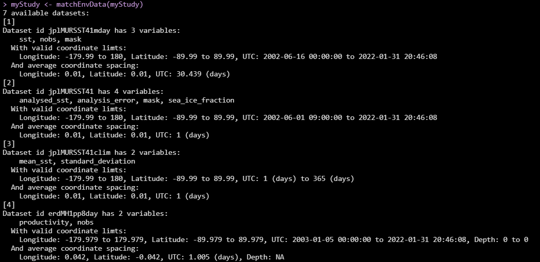
Each dataset has an ID (this is usually the exact ERDDAP ID, which may not be particularly informative), a list of variable names (also exactly matching the names as stored in the data structure, may not be informative), the range of valid coordinates (pay particular attention to time range if you are working with older data), and the average spacing of the coordinates (note the jplMURSST dataset has three flavors with different time spacing - daily, monthly, and averaged climatology).

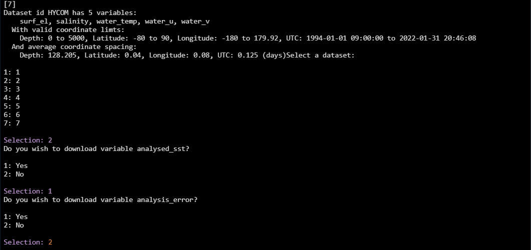
Choose which one you want by entering the appropriate number, then you will be asked which of the variables you want to download. Here we download the daily MURSST data (#2), and then choose to download only the analysed_sst variable, selecting “No” analysis_error, mask, and sea_ice_fraction (click image for larger view):

After making decisions for all the variables, the data will start to try and download, and you will see a progress bar. If the temporal and phyiscal range of your dataset is small, this can be quite quick, but for larger datasets it might take some time. PAMpal tries to break up larger downloads into smaller individual chunks since most servers have limits on file size. Note that download from HYCOM servers usually involve longer delays.

What Did We Download?

So, what does this function actually do? For each AcousticEvent in your AcousticStudy, matchEnvData will get the environmental data closest to the coordinate associated with the start of that event. This means that each event will have a single piece of environmental data associated with it, rather than a separate value for every single detection within that event. This is because environmental variables typically change on a much larger scale than individual detections within an event, but if you have exceptionally long events this might not be the most accurate (there are other options you may try further below).

NOTE Currently (01/31/2022 / v0.15.1) if your environmental dataset has a Depth component, matchEnvData will average the value over all available depths. This is changed in v0.15.2 and later (currently on GitHub not yet on CRAN), in these versions you can specify a depth argument to set the depth you need or range of depths to average over (ex. depth=0 to get surface value, depth = c(100, 400) to average over depths between 100m and 400m).

To see the data, you can use the getMeasures function. The measures are special values stored for each event so that PAMpal knows to export them for modeling applications, so you might also see the ICI or some other things here depending on what other processing you have done. The measures will also be attached to your detections when using the getDetectorData family of functions (as of PAMpal v0.15.2, not yet on CRAN as of 01/30/2022 only on GitHub). You’ll also note that each variable name has _mean appended to the end, this refers to the default summarising function mean applied to the environmental data, see the section on summarising data over a range below.

# You should see the downloaded values here for each event
getMeasures(myStudy)
# This should have a new column for the environmental data
str(getClickData(myStudy))

There is also one more place the environmental data is stored, in the ancillary slot of each AcousticEvent. This is a spot in each event that stores a lot of different things from different places, and is not used for exporting to models like the measures are. However, there is more information stored here that you may wish to use for troubleshooting. You will notice that there are a few more values stored here for each piece of environmental data. In additional to the normal variable names, there are columns for matchLat, matchLong, and matchTime. The Netcdf files have fixed datapoints, so these tell you the coordinate within the Netcdf file that your data matched to. This can be useful to double check and make sure that matches were made appropriately, or in cases where your Netcdf file did not fully cover the range of your data.

# Look at more detailed info for first event
ancillary(myStudy[[1]])$environmental

Download Other ERDDAP Datasets

If you have a different ERDDAP dataset in mind, PAMpal can also work with that. If the dataset is on the upwell server, then you can just provide the dataset id as the nc argument, and then it will ask which variables you want as before:

myStudy <- matchEnvData(myStudy, nc='erdMWpar01day')

If it is on a different server, there is slightly more set-up involved, and you may need to manually load the PAMmisc package for the rest to work. You will need to set up an edinfo object using the function erddapToEdinfo. This object contains all the info needed to create the server request that lets PAMpal sort out the downloading process for you. Here we’ll create one for this distance to shore dataset stored on a different ERDDAP server. We need to tell it the dataset ID and the URL of the dataserver. It will then ask which variables you want to download, as before.

library(PAMmisc)
# dataset is the dataset ID
# baseurl is the rest of the URL, up to /erddap/
dist2shore <- erddapToEdinfo(dataset='dist2coast_1deg'
                             baseurl='https://pae-paha.pacioos.hawaii.edu/erddap/')
# Then use this as the "nc" argument
myStudy <- matchEnvData(myStudy, nc=dist2shore)

Download Without Interactive Steps

While PAMpal’s interactive features can be useful when doing an exploratory analysis, or for one-off analyses, it can be a hassle for any analysis that might get run multiple times and is not ideal for reproducibility since the code itself leaves no clues as to what actually happened. Getting environmental data without any interactive steps just requires us to know the names of the variables we want. If a dataset is on the upwell ERDDAP server, the variable name can be given to matchEnvData as the var argument.

# This dataset is on upwell, we'll select the sst variable by name
myStudy <- matchEnvData(myStudy, nc='jplMURSST41', var='analysed_sst')

If the dataset is on a different server, or we need to create the edinfo object separately for some other reason, then we can supply the variable names to the erddapToEdinfo function as the chooseVars argument.

# this dataset is on a different server, we want the distance variable "dist"
dist2shore <- erddapToEdinfo(dataset='dist2coast_1deg',
                             baseurl='https://pae-paha.pacioos.hawaii.edu/erddap/',
                             chooseVars = 'dist')
myStudy <- matchEnvData(myStudy, nc=dist2shore)

Saving the Downloaded File

If you need to re-use the same environmental dataset for multiple analyses, you might be able to save the file and use it instead of downloading the same dataset multiple times. Just setting the fileName argument will have PAMpal save the downloaded Netcdf file. However, there are situations where this doesn’t work. If your dataset covers a large range of times or locations, the file size required to download that all in a single file might be too large. The dataservers typically have restrictions on how large of a file they can serve, and if this happens this download will fail. Even if it doesn’t fail, it might take quite a long time. When not saving the downloaded file, PAMpal can get around this issue by breaking down the request into several smaller downloads, so if you are not able to save the Netcdf file then this is always an option.

# Save our distance to shore data for future use
myStudy <- matchEnvData(myStudy, nc=dist2shore, fileName='Dist2Shore.nc')

Loading From an Existing Netcdf File

If you were able to download your data as above, how can you actually use it? Easy! Just set the nc argument to that filename, and PAMpal will load in all the variables stored in that Netcdf file. Unlike when downloading, it will not ask which variables you are interested in, it will just take everything that is available. One potential issue here - Netcdf files do not have universal standards for how coordinates are stored, so it is possible that if you have a Netcdf file from somewhere else that it might not be able to read it properly. This is typically an issue with how the date/time information is stored - PAMpal can currently handle most of the formats found on ERDDAP, but if you encounter a problem here please reach out and I will get it fixed for you!

# Use the data we stored in the step above
myStudy <- matchEnvData(myStudy, nc='Dist2Shore.nc')

Summarising Environmental Variables Over a Range

Sometimes it can be useful to summarise environmental variables over a range of values instead of just picking the closest value. To support this, there is a buffer argument that can be used to set a range of values to summarise over. This is a vector of length 3 specifying how much to expand the Longitude, Latitude, and Time values in each direction (units of decimal degrees and seconds). For example if our point was at 32, -117:

# All values between Lat 30,34 and Long -118,-116
myStudy <- matchEnvData(myStudy, 'jplMURSST41', buffer = c(1, 2, 0))
# Average all times within one day
myStudy <- matchEnvData(myStudy, 'jplMURSST41', buffer = c(0, 0, 86400))

How are they summarised? By default, all values within the buffer range are averaged, but if you want to do something else like the median or come up with some other way to summarise you can provide these as a vector FUN. Each function creates another stored variable for each environmental variable as EnvVariableName_FunctionName

# Compute standard deviation as well as default mean
# Stored vars "analysedsst_mean" and "analysedsst_sd"
myStudy <- matchEnvData(myStudy, 'jplMURSST41', 
                        buffer = c(1, 1, 0), FUN=c(mean, sd))
# Replace mean with median
# Stored var "analysedsst_median"
myStudy <- matchEnvData(myStudy, 'jplMURSST41', 
                        buffer = c(1, 1, 0), FUN=c(median))

If you write your own summarising function, just provide the name of that to FUN. These functions should expect a matrix of values, and should expect the possiblity of NA values.

More Options for Dataframes

All of the above methods can work on dataframes instead of AcousticStudy objects, in which case every single row of the dataframe will get its own matching environmental data. This can be useful if you have exceptionally long events, you can extract a dataframe of your detections using the getDetectorData family of functions and then match environmental data to it.

library(PAMmisc)
clicks <- getClickDat(myStudy)
clicks <- matchEnvData(clicks, 'jplMURSST41')

You will notice that when matching to a dataframe there are a lot more columns attached. In additional to the normal variable names, there are columns for matchLat, matchLong, and matchTime. The Netcdf files have fixed datapoints, so these tell you the coordinate within the Netcdf file that your data matched to. This can be useful to double check and make sure that matches were made appropriately, or in cases where your Netcdf file did not fully cover the range of your data. These columns can be removed from your output by setting keepMatch = FALSE

Filtering Data

AcousticStudy objects can be filtered with syntax similar to the dplyr package using the function filter. There are currently five ways data can be filtered: by database, species, environmental data values, detector name, and function parameter values.

Filtering by database leaves only events with databases in files(event)$db matching the criteria provided, but database names must exactly match the full file path to the database. Criteria are specified using either database or Database, the best way to provide the full names is typically by indexing from files(myStudy)$db. Alternatively, functions like basename can be used

# This won't work because it needs the full file name and path
oneDb <- filter(myStudy, database == 'FirstDb.sqlite3')
# This works instead, events from only first database
oneDb <- filter(myStudy, database == files(myStudy)$db[1])
# This also works
oneDb <- filter(myStudy, basename(database) == 'FirstDb.sqlite3')
# Events from all databases other than first
notFirstDb <- filter(myStudy, database != files(myStudy)$db[1])
# To specify multiple, use %in%
# Events with first two dbs only
twoDb <- filter(myStudy, database %in% files(myStudy)$db[1:2])
# Events from all dbs other than first two
notTwoDb <- filter(myStudy, !(database %in% files(myStudy)$db[1:2]))

Filtering by species leaves only events matching the species criteria provided, and thus should only be done after species are assigned using setSpecies. Criteria are specified using either species or Species.

# Only 'ZC' events
zcOnly <- filter(myStudy, species == 'ZC')
# Not ZC events
notZc <- filter(myStudy, species != 'ZC')
# To specify multiple species, use %in%
ZCGG <- filter(myStudy, species %in% c('ZC', 'GG'))
notZCGG <- filter(myStudy, !(species %in% c('ZC', 'GG')))

Filtering by environmental data leaves only events matching the criteria provided, and the names of the criteria must exactly match the names of variables listed in ancillary(myStudy[[1]])$environmental, so it is usually best to double check these names before filtering.

# This probably wont work because name is not exact match
shallowOnly <- filter(myStudy, sea_floor_depth > -500)
# Environmental parameters usually have mean or median added to the name, this works
shallowOnly <- filter(myStudy, sea_floor_depth_mean > -500)

Filtering by detector name leaves only detections from detectors matching the criteria provided, and the names of the criteria must exactly match the names of detectors. Note that Click Detectors typically have a number appended to their name, and all detectors use underscores instead of spaces. Note that these also take their names from the names given in Pamguard, which may not always be the default. It is best to check exact names using names(detectors(myStudy[[1]])) before filtering. Any events left with no detections will be removed from the study.

NOTE This has changed in PAMpal v0.17.0. Previously you used “detector” to filter by detector, now you use “detectorName”

# Remove Click_Detector_0
noZero <- filter(myStudy, detectorName != 'Click_Detector_0')
# Just 1 or 2
justOneTwo <- filter(myStudy, detectorName %in% c('Click_Detector_1', 'Click_Detector_2'))

Filtering by function parameters works slightly differently than the above four methods. The interface is the same, but instead of removing entire events it will remove all detections that do not match the criteria supplied. Parameter names must exactly match the names of parameters calculated by some of the processing functions. If a name provided does not match the name of a parameter in a detector, then all of that data will remain unfiltered. For example, trough is a value measured by standardClickCalcs, so filtering by trough > 10 will affect all click detections in your data, but will leave all Whistle or Cepstrum detectors untouched. Any events that are left with 0 detections after filtering are removed.

less10Peak <- filter(myStudy, peak < 10)
peak10to20 <- filter(myStudy, peak > 10, peak < 20)

Multiple types of filters can also be combined into a single filter statement

filterStudy <- filter(myStudy,
                        database != files(myStudy)$db[3],
                        species == 'OO',
                        sea_floor_depth_mean < -1000,
                        peak > 15)

If you want to filter out specific events by event id / event name, that is actually easiest to accomplish without using the filter function at all, but rather just using [] to subset your data. You can provide either indexes or full event names, event names are usually easiest to provide by indexing into names(events(myStudy))

firstOnly <- myStudy[1]
someOdds <- myStudy[c(1,3,5,7,9)]
byName <- myStudy[names(events(myStudy))[c(1,3,5)]]

KNOWN ISSUES WITH FILTERING

Currently there are two known issues with the filter function as implemented. First, if you supply a long list of options for a single filter, it won’t work and will likely give you an error. As a workaround, the function works fine if you first assign these to a variable, then filter.

# This probably won't work
badFilt <- filter(myStudy, species %in% c("SPECIES1", "SPECIES2", "SPECIES3", "SPECIES4", "SPECIES5",
                             "SPECIES6", "SPECIES7", "SPECIES8", "SPECIES9", "SPECIES10"))
# This should be fine
mySpecies <- c("SPECIES1", "SPECIES2", "SPECIES3", "SPECIES4", "SPECIES5",
                "SPECIES6", "SPECIES7", "SPECIES8", "SPECIES9", "SPECIES10")
goodFilt <- filter(myStudy, species %in% mySpecies)

Second, the filter function currently does not behave well if you try to use it inside other functions. Unfortunately there is not currently a work around for this, but I will be looking into improving the function in the filter so that these issues do not occur.

# This probably won't work
myFilter <- function(x, sp) {
    filter(x, species %in% sp)
}
# running this will give an error about "object 'sp' not found"
myFilter(myStudy, 'SPECIES1')

Accessing Binary Data

Sometimes it can be useful to access the binary data that PAMpal uses when initially processing data, especially if you need access to the wave forms of click detections. PAMpal has a function getBinaryData that makes this easy. You just need to provide the UIDs of detections that you would like binary data for, and the binary data for each will be returned in a list. There are occasionally instances where UIDs can be repeated across different types of detectors, so there is also a type argument that you can use to specify whether you are looking for binaries from clicks, whistles, or cepstrum detections, although this is usually not needed. Typically the easiest way to get UIDs without copying/pasting is with getDetectorData or the similar functions getClickData, getWhistleData, and getCepstrumData.

# Get the UIDs first to make things easier, then get click binary data
clickUIDs <- getClickData(myStudy)$UID
# These are usually identical, but occasionally it is necessary to specify type
binData <- getBinaryData(myStudy, UID=clickUIDs)
binData <- getBinaryData(myStudy, UID=clickUIDs, type='click')
# plot the waveform of the first click
plot(binData[[1]]$wave[, 1], type='l')

Exporting for BANTER Model

If you’ve ever tried to run a model created by someone else on your own data, you probably know that just getting your data formatted properly can be a huge challenge. One of our goals with PAMpal is to reduce that headache by creating export functions that will organize your data into the format required by various models. Currently we only support exporting data for creating BANTER models (see: package banter available on CRAN, BANTER paper, BANTER guide). In the future we hope to add support for a variety of models, feel free to e-mail me at taiki.sakai\@noaa.gov if you have a model that you would like to have supported.

Exporting data in your AcousticStudy object is as easy as calling export_banter. The output is a list with events, detectors, and na. The contents of events and detectors are formatted for banter::initBanterModel and banter::addBanterDetector, respectively, and na is a dataframe showing the information for any detections that had NA values (these will be removed from the exported data since random forest models cannot deal with NAs). Also note that BANTER can use event-level information in addition to information about each detection. Of PAMpal’s provided functionality, currently only calculateICI and matchEnvData will add this kind of event-level information to your AcousticStudy object, but in general anything that is in the list named measures in the ancillary slot of each event can potentially be exported for modeling purpose (you can see this for your first event with ancillary(myStudy[[1]])$measures. Only event-level measures that exist for all exported events can be used in a BANTER model, export_banter will issue a warning message if there are event-level measures found that are not present in all events.

# Assign species labels before exporting so that data can be used to train a model
myStudy <- setSpecies(myStudy, method='pamguard')
banterData <- export_banter(myStudy)
names(bnt)
# create model using exported data.
banterModel <- banter::initBanterModel(banterData$events)
banterModel <- banter::addBanterDetector(banterModel, banterData$detectors, ntree=50, sampsize=1)
banterModel <- banter::runBanterModel(banterModel, ntree=50, sampsize=1)

# add ICI data for export
myStudy <- calculateICI(myStudy)
# This may issue a warning about event-level measures depending on your data
banterICI <- export_banter(myStudy)

export_banter will issue warning messages if any of the species or detectors have an insufficient number of events (see BANTER documentation for more information about requirements for creating a model), and it will also print out a summary of the number of detections and events for each species after running (this can be turned off with verbose=FALSE). There are also two parameters that will allow you to easily remove a subset of species or variables from the exported data, dropVars and dropSpecies. Both take in a character vector of the names of the variables or species that you do not want to be exported.

# dont include peak3 or dBPP in the exported variables
lessBanter <- export_banter(myStudy, dropVars = c('peak3', 'dBPP'))
# dont include species Unid Dolphin or Unid BW in exported
noUnids <- export_banter(myStudy, dropSpecies = c('Unid Dolphin', 'Unid BW'))

Finally, export_banter also has a logical flag training to indicate whether or not the data you are exporting is to be used for training a new BANTER model. If training=TRUE (the default), then species IDs are required for each event, but if it is FALSE then they are not required. Additionally, if training is a numerical value between 0 and 1, then the exported data will be split into $train and $test datasets, where the value of training indicates the proportion of data to use for a training dataset, with the rest being left in $test. Note that splitting your data into training and test sets is not actually needed for BANTER since it is based on a random forest model (ask Eric Archer if you need convincing), but the option is included since it is frequently asked for.

trainTest <- export_banter(myStudy, train=0.7)
names(trainTest)
nrow(trainTest$train$events)
nrow(trainTest$test$events)

Plotting Call Presence or Density Summaries

This is a longer topic with its own page

Working With .wav Files

While most of the functionality of PAMpal comes from reading and processing the data contained in the PAMguard binary files, there are some times when users need to work with the wav files directly. Typically this can be quite annoying to do since you need to match each detection to its corresponding wav file with timestamps, but PAMpal provides some functions to make this easier.

Adding Recording Files

The first step to letting PAMpal work with any wav files is to use the addRecordings function to add a map of the recording files to your AcousticStudy object. If you are working with a single database of detections, you simply provide the path to the folder containing your recording files as the folder argument.

myStudy <- addRecordings(myStudy, folder='path/to/recordings')

If you have Soundtrap recordings, you can also provide the XML log files to this function. Sometimes there are gaps or recording error information stored in the log files, and this will help PAMpal sort that out.

myStudy <- addRecordings(myStudy, folder='path/to/recordings',
                         log = 'path/to/logs')

If your AcousticStudy covers multiple databases, then you will need to provide a separate recording folder for each database. It is common for users to have deployments that overlap in time, so this is what allows PAMpal to decide which wav file a detection belongs to in these cases. Here folder should be a vector of folder paths, one for each database. The order of these should match the order of files(myStudy)$db.

# check order first
files(myStudy)$db
recFolders <- c(
    'path/to/db1recordings',
    'path/to/db2recordings'
    )
myStudy <- addRecordings(myStudy, folder=recFolders)

The addRecordings function will go through your folder(s) of wav files and determine the start and end time of each file. These will be stored in a dataframe within your AcousticStudy object in files(myStudy)$recordings. This function has to open the header information of every single wav file to determine the exact file length, so it can take quite a bit of time.

Using Recording Files

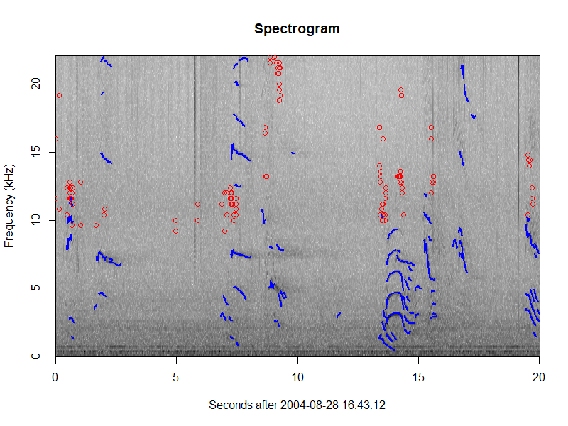
Once files have been added with addRecordings, some extra PAMpal functionality is opened up. One new function is plotGram, which allows users to plot spectrograms of their events. This reads in data from the wav files to create a spectrogram of a specified duration (or an entire event). It also allows users to overlay click detections (as circles), whistle contours, and cepstrum detection contours.

plotGram(myStudy, evNum=1, start=0, end=20, detections=c('click', 'whistle'), detCol=c('red', 'blue'))

There are also functions that allow users to access clips of wav data associated with their detections or events. getClipData returns a list of WaveMC class objects from the tuneR package, either for each event (mode='event') in the data or for each detection (mode='detection'). Users can also specify a buffer to extend the clip length before and after the desired event/detection. If buffer is a single value, then clips will be extended by that amount before and after the clip, so buffer=1 adds one second before the clip and one second after. Alternatively, if buffer is a vector of length 2 then separate values will be used before and after (first number should typically be negative). So buffer=1 is identical to buffer=c(-1, 1).

# create clips of each detection, padding by half a second on each side
clips <- getClipData(myStudy, buffer=c(-.5, .5), mode='detection')

There is also a channel argument if the original wav files are multichannel, this specifies which channel to use. There is also a useSample option that can be useful if extremely precise times are necessary (e.g. if trying to create clips of echolocation clicks). PAMguard typically stores times to millisecond accuracy, but sometimes this is not accurate enough. There are also detection times stored as sample numbers in the binary files, and PAMpal will try to use these if useSample=TRUE. The downside is that this takes longer, and there are occasions where it does not work properly if there is not enough recording information in the database (issues are typically related to data processed with the “Merge contiguous files” option checked in PAMguard, and will result in warnings when addRecordings is run). For most use cases useSample=FALSE is fine and recommended.

getClipData also has a FUN argument that lets users apply a function to each wav clip instead of just returning the clip. FUN optional function to apply to wav clips. This function takes default inputs wav, a Wave class object, name the name of the detection or event, time the start and end time of the clip, channel as above, mode as above, and additional named arguments can be passed to getClipData.

# custom function to print name and length of each wav file while returning clip
# with an extra "message" argument
nameLen <- function(wav, name, time, channel, mode, message) {
    print(paste0('Length (samples): ', length(wav@.Data[, 1]),
                 ' for ', name, ' message ', message))
    wav
}
clips <- getClipData(myStudy, FUN=nameLen, mode='detection', message='test!')

A special case of this FUN functionality is implemented with the writeEventClips function. This function will write wav clips to disk of either entire events or each detection. It uses all the same arguments as getClipData, with a couple extras. outDir specifies the directory that the clips should be written to. filter allows users to specify a low-pass, high-pass, or band-pass filter. A value of 0 applies no filter. A single value applies a highpass filter at that value. A vector of two values applies a lowpass filter if the first number is 0, or a bandpass filter if both are non-zero. All filter values are supplied in units of kHz.

File names are returned by writeEventClips, and files are formatted according to this: [Event or Detection][Id]CH[ChannelNumber(s)][YYYYMMDD][HHMMSS][mmm].wav The last numbers are the start time of the file in UTC, accurate to milliseconds. The Id is either the event ID or the detection UID. A helper function parseEventClipName is included that can take in one of these file names and return either the event/detection ID or the file time.

# create clips of each detection, applying a 20kHz low-pass filter
# Clips are written to the current directory
clipFileNames <- writeEventClips(myStudy, buffer=c(-.5, .5), 
                                 filter=c(0, 20), mode='detection', outDir='.')
# get start time of first clip
parseEventClipName(clipFileNames[1], part='time')